Revised Bottom Pressure Dedrifting

Bottom pressure recorders are subject to drift, with an exponential component over a period of months and a longer term linear change. The drift can vary between neighbouring instruments and even between redeployments of the same sensor (Watts and Kontoyiannis, 1990; Polster et al., 2009).

The standard procedure, as currently applied to all the records on this site, is to fit a drift function of the form \[p_\mathrm{drift}=a_1+a_2\tau+a_3\mathrm{e}^{-\tau/|a_4|}\] where \(\tau\) is the time in days since the start of the deployment.

However the bottom pressure sensor is also correctly recording both a long-term linear trend and annual and interannual signals, and the fit of a function of this form is particularly sensitive to the timing of the deployment relative to the annual cycle. We can improve the accuracy of the drift function by first removing all known annual and other long period functions, such as the pole tide.

The procedure was first described in Hughes, Christopher W.; Tamisiea, Mark E.; Bingham, Rory J.; Williams, Joanne. 2012 Weighing the ocean: Using a single mooring to measure changes in the mass of the ocean. Geophysical Research Letters, 39 (17). L17602.10.1029/2012GL052935 and is explained in more detail in Williams, J.; Hughes, C.W.; Tamisiea, M.E.; Williams, S.D.P.. 2014 Weighing the ocean with bottom-pressure sensors: robustness of the ocean mass annual cycle estimate. Ocean Science, 10 (4). 701-718.10.5194/os-10-701-2014

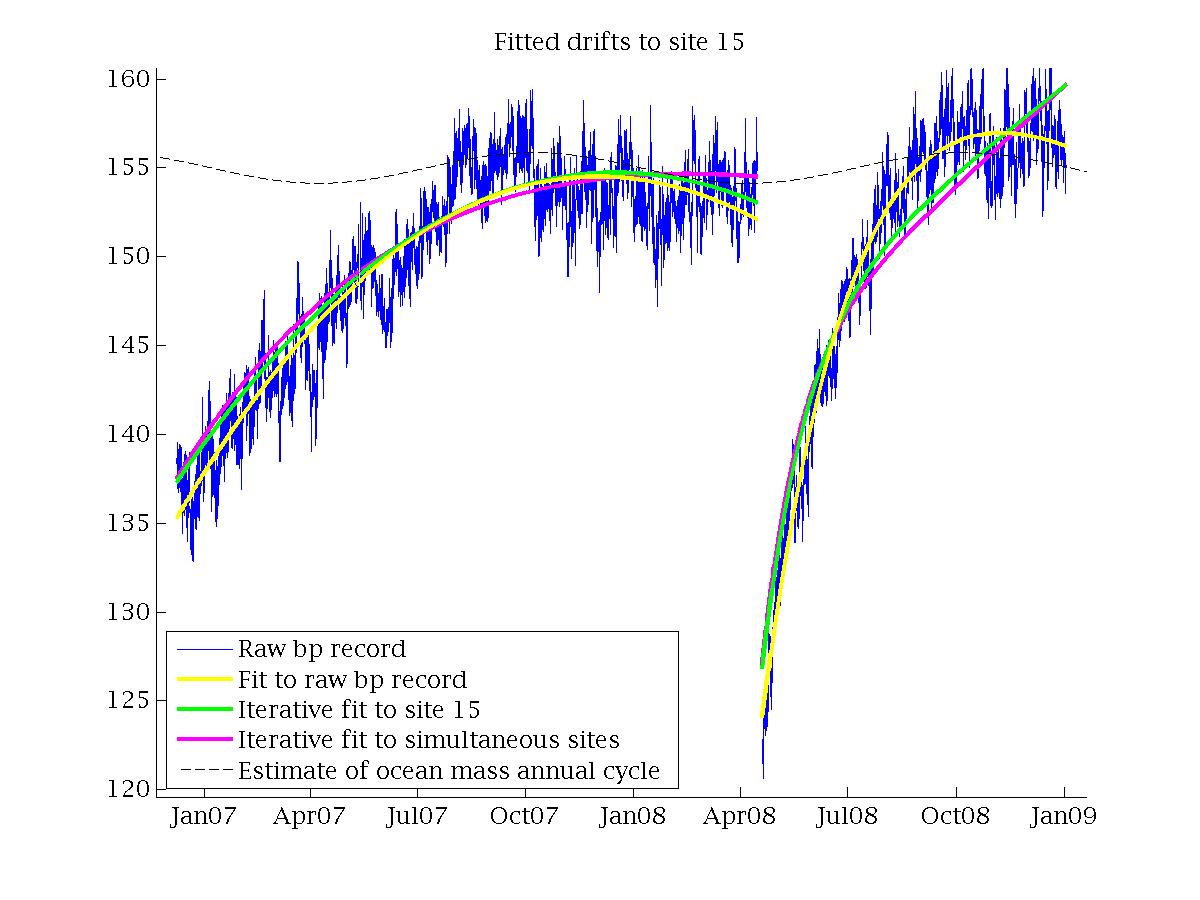
Example of an iterative fit to a bottom pressure record

Figure 3 from that paper provides a clear example from a site in the west Pacific. The apparent decrease of the bottom-pressure record in late 2008 is due to the coincidence of the annual ocean mass decrease. The drift fitted to the raw data is \(21.54-0.05\tau-47.47e^{-\tau/84.33}\), which is decreasing at the end of the record. The iterative fit allows for the sinusoidal contribution of the ocean mass and other variables, and the resulting drift is \(-3.76+0.05\tau-19.41e^{-\tau/37.24}\), increasing throughout the record. Using the raw-data drift fit would result in a bottom pressure error of over 3 mbar for the end of the record. With a differing sign for the linear part, serious error could result from any extrapolation of the raw-data drift fit.

Although we have so far chosen to keep to the widely understood simple dedrifting for the data provision, we provide here Matlab code and the necessary data to carry out this dedrifting. Users are requested to credit PSMSL and cite Williams et al. 2014 or Hughes et al 2012.

Note that this code requires the Matlab Optimization Toolbox. It can be altered to be used with the Matlab Statistics Toolbox instead, although the fitting algorithm is not as robust. See the help text in PSMSL_dedrift.m for further information.

Once again, we must emphasise that this technique can not possibly separate the linear part of the recorder drift from linear trends, so recorders subject to this drift can not be used to derive sea-level trends.

Data

Revised Bottom Pressure Dedrifting