Jump to main content.

•    About Us   
•    Data   
•    Products   
•    GLOSS   
•    Training   
•    Links   

You are here: home > products > trends >

Methods used for fitting trends

In 2015, we changed the method used to calculate fitted trends. Primarily, this was done to allow the calculation of realistic uncertainties, but at the same time we also began to use our monthly, rather than our annual data set.

Previously, trends were calculated using a simple linear regression. However, this method is unsuitable for calculating uncertainties in trends, as the observations in the series are not totally independent of each other. In order to attempt to account for this autocovariance, trends are now fitted using an Integrated Generalized Gauss Markov stochastic model (see below for a full description).

The data

The data selection method remains the same as before:

• Only RLR data are used, as Metric data have no long term datum control. See our help file for an explanation of these terms.
• Trends are only calculated where a station has at least 70% of annual means present over a given period.
• Trends are not calculated for stations which have been marked with a quality control flag.
• Data marked with a quality control flag are ignored, and are treated as missing.

Note that although the trends are fitted to monthly data, selection occurs using the annual data, ensuring that the data properly represents the annual cycle.

The model

For each period fitted, the time series is decomposed into the following components:

• A linear trend
• A seasonal component - made up of an annual and a semi-annual cycle
• The noise component - modelled using three stochastic parameters and an amplitude, and a white noise amplitude (see below)

The weighted least squares parameters are calculated using maximum likelihood estimation.

The procedure

For each station, the following procedure occurs:

• The longest available window with 70% of annual data present is identified.
• The Generalized Gauss Markov Model is fitted over this window. The stochastic noise parameters of this model are stored.
• Models are fitted over all other possible combination of start and end years that satisfy 70% completeness over 30 or more years. The stochastic noise parameters from the original model are used to derive the covariance structure in the weighted least squares equations.

Note that no attempt has been made to assess the appropriateness of the linear regression model for any given fit. Rather, values have been calculated to illustrate global and regional trends. Therefore, individual values should not be treated as a research quality product suitable for publication, or for use in planning or policy making.

Should you wish to further investigate the trend at a particular site, we would invite you to download the RLR data and examine the relevant station documentation.

The Stochastic Model

Sea level varies on time scales from seconds to millions of years as a result of a wide variety of physical processes [Harrison, 2002]. Hughes and Williams [2010] highlighted the importance of spatial variations in the spectral shape of sea level using satellite altimeter data.

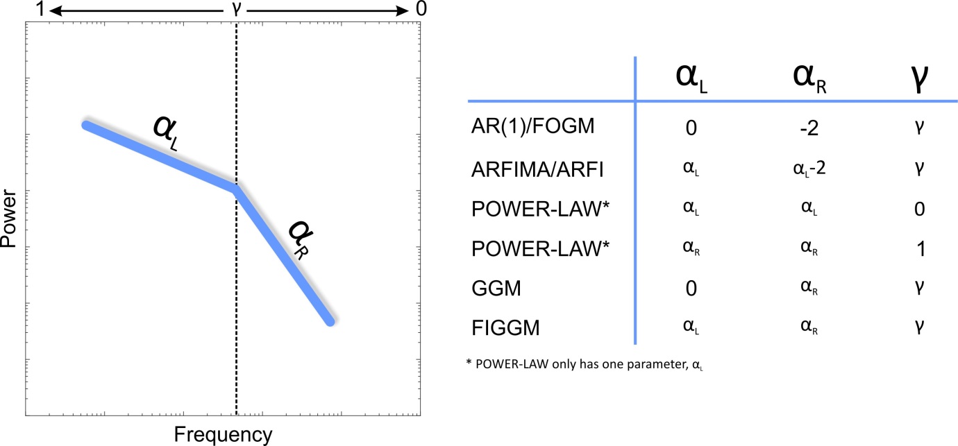
Bos et al [2014] also showed the variety in temporal correlations in sea level using PSMSL tide gauge data. They used a range of stochastic models such as white noise, Autoregressive noise (both AR(1) and AR(5)), Autoregressive Fractionally Integrated (ARFI) noise and Generalized Gauss Markov (GGM) Noise. Rather than use multiple stochastic noise models we introduce a new, more general model, which requires three parameters, α_L, α_R and γ. This model is shown pictorially in the figure below as an idealized power spectrum plotted in log-log space. A Fractionally Integrated Generalized Gauss Markov (FIGGM) model has two regions separated at some frequency, f_c, which is related to the AR(1) parameter, γ. To the left of f_c, the spectrum has a slope in log-log space equal to α_L and a slope of α_R to the right of f_c. All of the other models can be considered special cases of FIGGM. For instance AR(1) (also called First-Order Gauss Markov (FOGM) noise) simply has one parameter, γ, which describes where the break point is; α_L is 0 and α_R is -2. Power-law noise which simply has one slope can arise from a number of combinations of the three parameters. We estimate all three parameters together with the amplitude for the noise and the amplitude for a white noise component (spectrum will flatten at high frequencies). Using a FIGGM stochastic model means that the form of the noise in the data can take on that of any of the other models without implicit forcing of the parameters.